How to Interpret Cronbach's Alpha: What the Number Says and When It Lies

Cronbach's alpha takes a minute to compute and about as long to misread. A 0.85 does not prove that your questions measure one thing, a 0.65 does not condemn a scale on its own, and a negative value almost never reflects on the questions. It reflects on how the data was coded.

The definition lives in our glossary entry on Cronbach's alpha. This article starts where the calculation ends: which values count as acceptable, when the number misleads, and how to get it in Excel, SPSS, R or Python.

What Cronbach's alpha measures, and what it does not

Alpha answers one plain question: do these items move together closely enough to be added into a single score? If people who score high on one statement tend to score high on the others, alpha rises. If every question goes its own way, it falls. It measures internal consistency, one kind of reliability, and only makes sense when several questions are meant to measure the same thing and you plan to combine them into an index.

Alpha is not validity. Ten questions about the office coffee can come out highly consistent and say nothing about employee engagement, which is what you set out to measure. The coefficient confirms that the items share something. What that something is, you decide by reading the questions.

Nor does it prove that the scale measures a single thing (Cortina, 1993). And it is a property of the responses in front of you, not of the questionnaire, which is why you report the alpha from your own data rather than the one the scale's author published.

The Cronbach's alpha formula, piece by piece

The formula looks more intimidating than it deserves:

alpha = k / (k - 1) × (1 - sum of the item variances / variance of the total score)

Here k is the number of items, not the number of respondents. The sum of the item variances captures how much each question varies on its own. The variance of the total captures how much the summed score varies from person to person.

The trick is in the ratio. The variance of a sum includes the covariance of every pair of questions, so when the items move together, the variance of the total grows much faster than the sum of the separate variances. The ratio shrinks and alpha heads toward 1. With no relationship between the items, the two quantities nearly coincide and alpha sits around 0. If the items pull against each other more than they move together, it goes negative. The k / (k - 1) factor only rescales the result so that perfect consistency comes out as 1.

If all you need is the number, paste your responses into our Cronbach's alpha calculator. The rest of this article covers what the calculator cannot tell you: what the number means.

Now a small, illustrative example. Six people rate four statements about their last contact with technical support, from 1 (strongly disagree) to 5 (strongly agree): "My problem was solved," "I got a reply within a reasonable time," "The solution was explained clearly" and "I had to explain my problem more than once." The fourth is worded negatively, so the table already shows it recoded as 6 minus the original answer.

Respondent	Item 1	Item 2	Item 3	Item 4 (recoded)	Total
1	4	4	3	5	16
2	2	3	3	3	11
3	1	2	2	3	8
4	2	2	3	2	9
5	3	3	4	4	14
6	3	4	3	4	14
Variance (VAR.S)	1.1	0.8	0.4	1.1	10

The item variances add up to 1.1 + 0.8 + 0.4 + 1.1 = 3.4. Divided by the variance of the total, 10, that gives 0.34. One minus 0.34 is 0.66, and multiplied by 4 / 3 it becomes alpha = 0.88. Six people only show the mechanics. The calculator itself recommends at least 30 responses, and 100 or more for a stable estimate.

Cronbach's alpha values: what counts as acceptable

The answer comes from two sources that are best kept apart. The first is the rule of thumb in George and Mallery (2003), an SPSS handbook that countless theses cite:

Alpha	Label per George and Mallery (2003)	What to do in practice
0.9 or higher	Excellent	Above 0.95, look for repeated questions
0.8 to 0.9	Good	Solid for basic research
0.7 to 0.8	Acceptable	Enough for early-stage work
0.6 to 0.7	Questionable	Review the items before adding them up
0.5 to 0.6	Poor	Do not build the index yet
Below 0.5	Unacceptable	No scale, or an error in the data

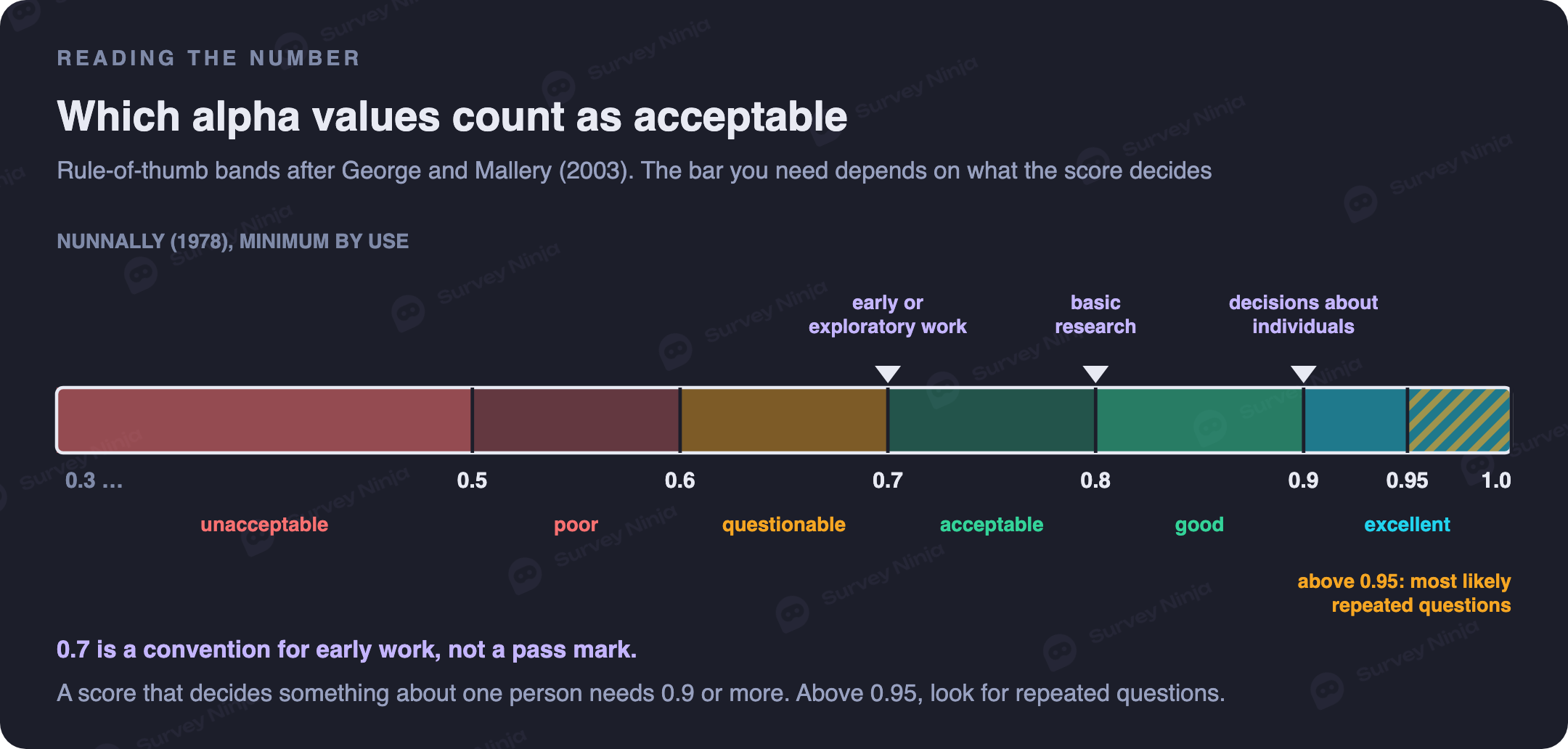
The second is Nunnally (1978), and the logic is different: the minimum depends on the use. In the early stages of research, 0.7 is enough. For basic research, 0.8. When the score feeds decisions about specific people, such as choosing between job candidates, 0.9 is the minimum to tolerate and 0.95 the desirable standard.

You will meet the same table with other adjectives. Some sources, calculators included, call the 0.6 to 0.7 band "acceptable." The cut points barely move. The words do, so name your source whenever a label goes into a report.

Why 0.7 is a convention, not a law

In many reports, 0.7 works like a pass mark: above it the scale is fine, below it the scale goes in the bin. Nunnally never framed it that way. He proposed that cutoff for the early stage of research and asked for considerably more as soon as the score was used for anything serious.

The number only makes sense with two facts beside it. One is the use. Comparing the means of large groups tolerates more error than a decision about one person, because individual errors tend to cancel out in an average. The other is the number of items. Three questions with an alpha of 0.68 can hang together more tightly than twenty with 0.82. With similar variances, the average inter-item correlation is about 0.41 in the first case and 0.19 in the second.

None of this turns a 0.55 into a good result. It only means the threshold is set before you see the data, and set by use.

More items, higher alpha: the length effect

From here on, the cases where the number misleads. The first is mechanical: alpha depends on how strongly the items are related and also on how many there are. Standardized alpha, which nearly matches ordinary alpha when item variances are similar, gives the exact relationship: k × r / (1 + (k - 1) × r), where r is the average correlation between items.

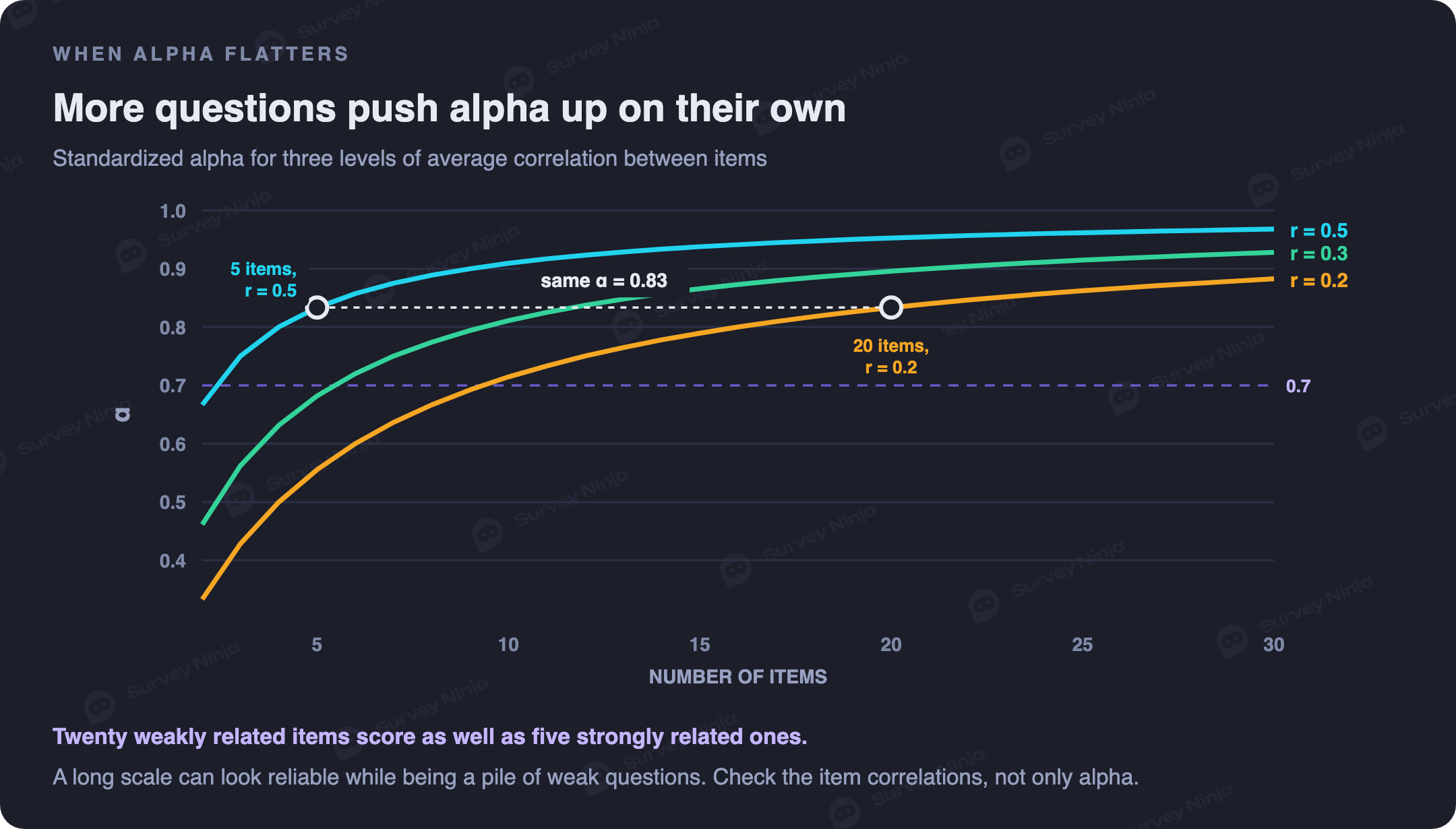
With a weak average correlation of 0.2, five items give 0.56, ten give 0.71, twenty give 0.83 and thirty give 0.88. At 0.3, five items give 0.68, ten 0.81 and twenty 0.90. At 0.5, five items already reach 0.83 and ten reach 0.91.

Look at the match. Twenty weakly related questions reach the same "good" 0.83 as five strongly related ones. Same number, different instruments. That is why an alpha without the item count beside it is half the information. It is also why shortening a questionnaire lowers alpha even when you cut no bad questions. Keep five of those twenty items, with the same average correlation, and alpha stops at 0.56.

Report the average inter-item correlation as well, since it does not depend on k. Clark and Watson (1995) suggest it should fall between 0.15 and 0.50.

Reverse-worded items and negative Cronbach's alpha

Many questionnaires include statements worded the opposite way so that nobody answers on autopilot, like "I had to explain my problem more than once." These get reversed before any calculation, as 6 minus the answer on a 1 to 5 scale and 8 minus the answer on a 1 to 7 scale. In general, the reversed score is the lowest plus the highest scale point, minus the answer.

Watch what happens if you forget. Take the original answers to the fourth statement (1, 3, 3, 4, 2, 2). The sum of the item variances stays at 3.4. But the variance of the total collapses from 10 to 2.4, because that question subtracts where the others add. The ratio climbs to 3.4 / 2.4 ≈ 1.42 and alpha drops to -0.56.

A negative alpha is not a very low alpha. It is a symptom, almost always of a reverse-worded item that nobody recoded. While you are there, check for codes such as 9 or 99 for "don't know." They do not always produce a negative value, but they distort any alpha. In small samples with nearly unrelated questions, a slightly negative value can also turn up by chance. Either way the message is the same. As they stand, those columns do not form a scale.

Our calculator will not even display a negative value. It asks you to check your data instead. SPSS does display it, with a footnote suggesting you check the item coding.

When a scale measures two things and still scores a high alpha

The opposite error is more dangerous because it makes no noise. Picture an engagement index built from twelve statements: six about working conditions and six about the relationship with the line manager. Suppose the items correlate at 0.5 within each block and at only 0.2 across the blocks.

Each block on its own gives an alpha of 0.86. All twelve statements together give practically the same, 0.86. Yet the two block scores correlate at just 0.34. They are close to being two separate measures. The overall coefficient does not show the seam, which is Cortina's (1993) warning in miniature.

The cost shows up in the report, where two teams with the same index score can have opposite problems. To catch it, check whether you can name in one word what the items measure. Look at the correlation matrix, where blocks jump out. If the scale matters, run a factor analysis. If two blocks emerge, calculate an alpha for each.

Above 0.95: questions that repeat each other

A sky-high alpha looks like the best possible news, and often it is not. Streiner (2003) cautions that past roughly 0.90, a higher alpha is more likely a sign of duplicated content than of a homogeneous scale. In the diagram, the caution zone starts at 0.95 because the 0.90 to 0.95 range is where Nunnally's standard for decisions about individuals sits, usually met by long tests. Above 0.95, not even that use asks for more.

In a survey, the usual culprit is paraphrase: "I am satisfied with the service," "The service leaves me satisfied," "My satisfaction with the service is high." Three questions, one piece of information. Keep the clearest wording and spend the freed slot on another facet. If writing it is the hard part, the question generator drafts questions from a topic.

How to read alpha if item deleted

SPSS and R both produce a table with one row per item and two key columns: the corrected item-total correlation, meaning each item's correlation with the sum of the others, and the alpha the scale would have without that item. SPSS calls them Corrected Item-Total Correlation and Cronbach's Alpha if Item Deleted. In R's psych package they are r.drop and raw_alpha. With the support data, already recoded:

Item	Corrected item-total correlation	Alpha if item deleted
1. My problem was solved	0.92	0.77
2. Reply within a reasonable time	0.85	0.80
3. Solution explained clearly	0.45	0.94
4. Had to explain my problem more than once (recoded)	0.80	0.82

Read it against the overall alpha of 0.88. If alpha falls when an item is removed, that item is holding the scale up, as items 1, 2 and 4 are. If it rises, the item weakens the scale. Item 3 is the candidate. It has the lowest correlation, and without it alpha would climb to 0.94.

Do you drop it? Not automatically. With six responses the difference proves nothing, clarity is a legitimate part of the support experience, and 0.94 is already brushing the zone of repeated questions. Deleting items until alpha is squeezed dry on the same sample leaves you with an optimistic number. Drop an item when the data and the content point the same way, then confirm it on fresh responses.

The table also gives away items that were never recoded. If the fourth statement keeps its original answers, its item-total correlation is -0.80 and alpha without it is 0.82, against -0.56 for the full scale. The calculator does not produce this table, but you can rebuild the column by dropping one item at a time. For an item's correlation with the sum of the rest, use the Pearson correlation calculator.

How to calculate Cronbach's alpha in Excel, SPSS, R and Python

Three preparations apply to any tool. Recode the reverse-worded items. Decide how to handle incomplete responses and "don't know" answers. And look at how the answers are distributed. If almost everyone picks 5, the question barely varies and alpha usually drops even when the scale is sound. A quick pass of descriptive analysis catches this in minutes.

Excel has no function for alpha, but VAR.S and SUM are enough. With one row per respondent, one column per item and the example data in B2:E7:

Step	What you calculate	Formula
1	Each respondent's total	=SUM(B2:E2) in F2, copied down to F7
2	The variance of each item	=VAR.S(B2:B7) in B9, copied across to E9
3	The variance of the total	=VAR.S(F2:F7) in F9
4	Alpha, with k = 4	=4/3*(1-SUM(B9:E9)/F9)

With a different number of items, replace 4/3 with k/(k-1). Two classic mistakes: putting the number of respondents into k, and mixing VAR.S with VAR.P. Either function works as long as the same one is used on both sides. Mix them on our six respondents and 0.88 becomes 0.79 or 0.96, depending on which way round.

In SPSS, the path is Analyze > Scale > Reliability Analysis. Move the items into the list, leave the model on Alpha and, under Statistics, tick "Scale if item deleted." That produces the table from the previous section. Reverse-worded items are recoded beforehand with Transform > Recode into Different Variables.

In R, the alpha function of the psych package reports raw and standardized alpha, the average inter-item correlation and alpha with each item dropped, and warns you when an item correlates negatively with the scale as a whole. Its check.keys option reverses those items automatically. Use it with care, because sometimes the item is not reversed, just badly worded.

In Python, the cronbach_alpha function of the pingouin library takes the items as columns and returns alpha with its 95 percent confidence interval, which is revealing when responses are few. By hand, with pandas, it takes three steps: add up the column variances, take the variance of the row totals and apply the formula. One catch: pandas defaults to sample variance and NumPy to population variance, and mixing the two shifts alpha just as it does in Excel.

For the quick answer there is the calculator from the top of this article. Paste the columns from Excel, one row per respondent, and you get alpha with an indicative label. Remove rows with gaps first, because the calculator trims every row to the length of the shortest one. The calculation runs in your browser.

Where alpha fits in survey work

Alpha's natural territory is the multi-item Likert-type scale, whose answers are summed or averaged into an index. How to build one is covered in our Likert scale guide. You calculate it twice: in the pilot, to fix questions, and on the real sample, to report the reliability of what you are about to analyze.

Outside that territory it has no job. A single question, such as the NPS question, has no internal consistency, and neither does a checklist of reasons for canceling a subscription. Nobody expects the person who ticks price to tick support as well. Inside the territory, reliability matters downstream. An unreliable index caps the correlation it can show with other variables, as our guide to correlation in surveys explains.

The usual alternative is McDonald's omega. Alpha assumes every item carries the same weight, and when that is not true it tends to fall below the real reliability. Omega starts from a factor analysis and does not need the assumption. When the weights are similar, the two come out nearly identical. You can get omega from the omega function in R's psych package and from free programs such as jamovi and JASP.

The loop is short: create a survey for free, collect the responses, export them and paste the columns into the Cronbach's alpha calculator. The number comes out on its own. This article is for deciding what to do with it.

Frequently asked questions

What is an acceptable Cronbach's alpha value?

George and Mallery (2003) call alpha acceptable from 0.7, good from 0.8 and excellent from 0.9, with questionable, poor and unacceptable bands below 0.7. Nunnally (1978) sets the minimum by use: 0.7 for early research, 0.8 for basic research, and 0.9 to 0.95 for decisions about individuals.

What does a negative Cronbach's alpha mean?

That some items move against the rest. It is almost always a reverse-worded item left unrecoded. Reverse those answers (6 minus the answer on a 1 to 5 scale) and calculate again.

Does a high Cronbach's alpha prove that a scale measures one thing?

No. As Cortina (1993) showed, a scale mixing two related dimensions can still score a high alpha, especially a long one. To check, read the questions, look at the inter-item correlations or run a factor analysis.

How do you calculate Cronbach's alpha in Excel?

There is no built-in function. Take VAR.S of each item column, add them up, take VAR.S of the column of totals, and apply k / (k - 1) × (1 - sum of item variances / variance of the total), where k is the number of items.

What does Cronbach's alpha if item deleted mean?

It is the alpha the scale would have without that item. Lower than the overall alpha means the item contributes. Clearly higher means it weakens the scale. Even then, weigh its content and confirm the gain on another sample before dropping it.

What is the difference between Cronbach's alpha and McDonald's omega?

Alpha assumes all items carry equal weight. Omega starts from a factor analysis and lets the weights differ. With similar weights they almost coincide. When the weights differ, alpha tends to underestimate reliability and omega estimates it better.