 WooCommerce Post-Purchase Survey: 7 Questions, When to Ask and What to Do Next
Van Westendorp Price Sensitivity Meter: Pricing Survey Questions and a Worked Example
Market research  Mike Taylor Updated: Nov 11, 2026 Reading time ≈ 18 min
Contents
- The four questions of the Van Westendorp price sensitivity meter
- Worked example: from answers to curves
- The four price points and the acceptable range
- The Gabor-Granger method: price ladder and demand curve
- Van Westendorp or Gabor-Granger: which method when
- Who to ask and how many answers you need
- Checks before you trust the numbers
- Limits of a pricing survey
- How to run a pricing survey in SurveyNinja
- Frequently asked questions

The Van Westendorp price sensitivity meter is a pricing survey built on four questions: at what price a product feels too cheap, a bargain, expensive and too expensive. Cumulative answers turn into four curves, and the points where they cross give an acceptable price range. Below is a full worked example you can redo in a spreadsheet, followed by the Gabor-Granger method, which estimates demand at set prices.
Both methods measure stated willingness to pay. That is useful early, when you need a range to test before real customers see a price.
Key points
- The Van Westendorp price sensitivity meter asks at what price a product feels too cheap, a bargain, expensive and too expensive.
- Cumulative answers form four curves, and the acceptable price range runs from the Point of Marginal Cheapness (PMC) to the Point of Marginal Expensiveness (PME).
- Use Van Westendorp when you do not know the range yet, and Gabor-Granger when you have a shortlist of prices and need the one that brings in the most revenue.
- Plan at least 100 to 200 valid answers per segment, and drop respondents whose four answers are not in increasing order.
The four questions of the Van Westendorp price sensitivity meter
The method was introduced by the Dutch economist Peter van Westendorp in 1976, in a paper titled "NSS-Price Sensitivity Meter (PSM): A new approach to study consumer perception of price", published in the proceedings of the 29th ESOMAR Congress. The idea is simple: ask for four price thresholds and let the distribution of answers show where price stops feeling right.
| Threshold | Question | Answer format |
|---|---|---|
| Too cheap | At what price would [product] be so cheap that you would doubt its quality? | Number in your currency |
| Cheap (a bargain) | At what price would [product] be a bargain, a great buy for the money? | Number |
| Expensive | At what price would [product] start to feel expensive, so you would have to think before buying it? | Number |
| Too expensive | At what price would [product] be so expensive that you would not consider buying it? | Number |
Before the four questions, show a short, neutral description of the product: what it does, who it is for, what is included. Without it, each person prices a different product in their head, and the curves blend those products together.
Use an open number field where you can. A slider is faster to answer, but its range and starting position suggest what a normal answer looks like. That is the anchoring effect at work, and in a price survey it moves the very numbers you are trying to measure. If you do use a slider, make its range wide, start it at zero and keep it the same for everyone. Keep the question order fixed for all respondents too, and do not show any price before these four questions.
Worked example: from answers to curves
The dataset below is an illustrative example, not real data. Imagine a monthly subscription to a scheduling app, priced in USD. Twenty-two people answered the four questions. Copy the table into a spreadsheet and follow along.
| # | Too cheap | Bargain | Expensive | Too expensive |
|---|---|---|---|---|
| 1 | 5 | 10 | 20 | 30 |
| 2 | 8 | 12 | 18 | 25 |
| 3 | 5 | 8 | 15 | 18 |
| 4 | 10 | 15 | 25 | 35 |
| 5 | 8 | 10 | 20 | 25 |
| 6 | 5 | 10 | 12 | 15 |
| 7 | 10 | 12 | 20 | 30 |
| 8 | 5 | 8 | 12 | 18 |
| 9 | 12 | 15 | 25 | 40 |
| 10 | 8 | 12 | 20 | 25 |
| 11 | 5 | 10 | 18 | 25 |
| 12 | 12 | 18 | 25 | 30 |
| 13 | 8 | 10 | 15 | 20 |
| 14 | 5 | 12 | 20 | 30 |
| 15 | 15 | 20 | 30 | 40 |
| 16 | 8 | 12 | 18 | 30 |
| 17 | 5 | 8 | 15 | 20 |
| 18 | 15 | 18 | 25 | 35 |
| 19 | 8 | 10 | 20 | 30 |
| 20 | 10 | 12 | 25 | 35 |
| 21 | 20 | 15 | 10 | 30 |
| 22 | 10 | 25 | 20 | 30 |
Step 1. Drop answers that are out of order. For a valid respondent, too cheap < bargain < expensive < too expensive. Respondent 21 says $20 is too cheap but $15 is a bargain, and respondent 22 calls $25 a bargain and $20 expensive. Both go. That leaves 20 valid respondents, and every share below is out of 20.
Step 2. Build the four cumulative curves. List every price that appears in the answers: 5, 8, 10, 12, 15, 18, 20, 25, 30, 35, 40. For each price, count respondents:
- Too cheap at price P: people whose "too cheap" answer is P or higher. If someone says $10 is too cheap, then $8 is too cheap for them as well. This curve falls as price rises, which is why it is called inverted.
- Bargain at P: people whose "bargain" answer is P or higher. Also inverted, also falling.
- Expensive at P: people whose "expensive" answer is P or lower. This curve rises.
- Too expensive at P: people whose "too expensive" answer is P or lower. Also rising.
In a spreadsheet, with prices in column H and the "too cheap" answers in B2:B21, the falling curves are =COUNTIF(B$2:B$21,">="&$H2)/20 and the rising ones use "<=". Two helper curves complete the set: "not a bargain" is 100% minus "bargain", and "not expensive" is 100% minus "expensive".
| Price, $ | Too cheap | Bargain | Not a bargain | Expensive | Not expensive | Too expensive |
|---|---|---|---|---|---|---|
| 5 | 100% | 100% | 0% | 0% | 100% | 0% |
| 8 | 65% | 100% | 0% | 0% | 100% | 0% |
| 10 | 35% | 85% | 15% | 0% | 100% | 0% |
| 12 | 20% | 55% | 45% | 10% | 90% | 0% |
| 15 | 10% | 25% | 75% | 25% | 75% | 5% |
| 18 | 0% | 15% | 85% | 40% | 60% | 15% |
| 20 | 0% | 5% | 95% | 70% | 30% | 25% |
| 25 | 0% | 0% | 100% | 95% | 5% | 45% |
| 30 | 0% | 0% | 100% | 100% | 0% | 75% |
| 35 | 0% | 0% | 100% | 100% | 0% | 90% |
| 40 | 0% | 0% | 100% | 100% | 0% | 100% |
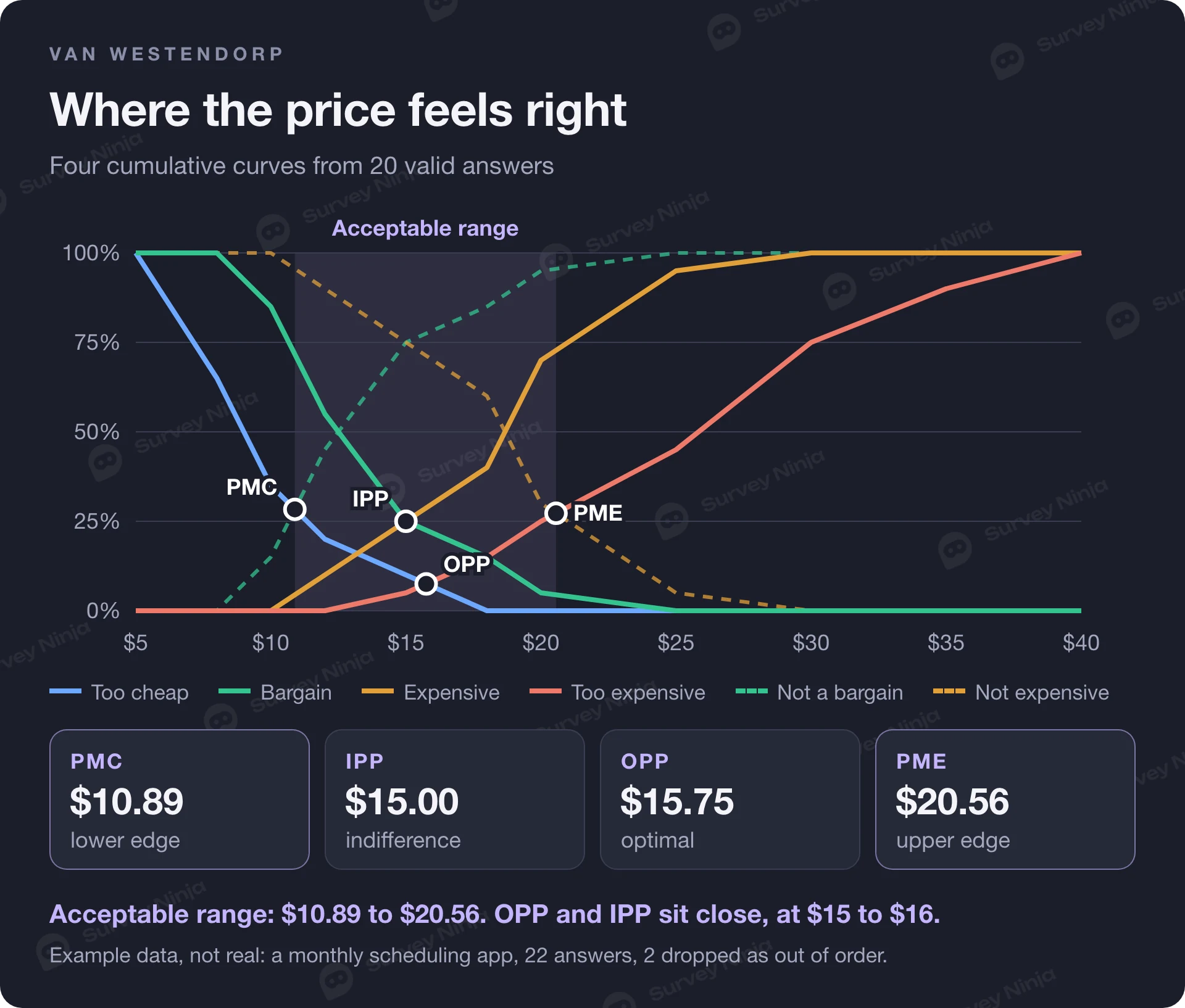
Step 3. Find where curves cross. A crossing usually falls between two listed prices, so interpolate linearly. Take the gap between the two curves at the lower price (d1) and at the higher price (d2). The crossing is at lower price + (higher price − lower price) × d1 / (d1 − d2).
For example, "too cheap" and "not a bargain" swap places between $10 and $12. At $10 the gap is 35 − 15 = 20 points. At $12 it is 20 − 45 = −25 points. The crossing is 10 + 2 × 20 / 45 = $10.89.
The four price points and the acceptable range
Each crossing has a name. With the original definitions, here is what the example gives:
| Point | Curves that cross | Example result | How to read it |
|---|---|---|---|
| Point of Marginal Cheapness (PMC) | Too cheap and not a bargain | $10.89 | Lower edge of the acceptable range. Below it, doubts about quality start to outweigh the appeal of a low price. |
| Optimal Price Point (OPP) | Too cheap and too expensive | $15.75 | Equal shares reject the price from each side. It is often read as the price the fewest people rule out, though that holds only roughly. |
| Indifference Price Point (IPP) | Bargain and expensive | $15.00 | As many people call the price a bargain as call it expensive. Often read as the price people see as normal for the category. |
| Point of Marginal Expensiveness (PME) | Too expensive and not expensive | $20.56 | Upper edge of the acceptable range. Above it, more people find the price out of reach than find it fine. |
The acceptable price range runs from PMC to PME, here $10.89 to $20.56. The OPP and IPP sit close together at $15 to $16. When the two are far apart, opinions about price are split, and that is worth a look by segment before you pick a number.
Check which convention your software or analyst uses. Some tools define the range with a narrower pair of crossings: "too cheap" with "expensive" and "too expensive" with "bargain". On the same data that gives $13.20 to $18.00. Both conventions appear in practice. The open-source pricesensitivitymeter package for R supports both and defaults to the original one used above. Name the convention in your report so nobody compares numbers built two different ways.
The Gabor-Granger method: price ladder and demand curve
Gabor-Granger answers a different question: what share of people would buy at each specific price, and which price brings in the most revenue? It was developed in the 1960s by the economists André Gabor and Clive Granger; one of their early papers is "On the Price Consciousness of Consumers" (Applied Statistics, 1961).
The setup is a price ladder: five to seven prices you would realistically charge. Each respondent sees one price and a purchase question such as "Would you buy [product] at $16 per month?" with a five-point scale from "definitely would not buy" to "definitely would buy". If they answer "probably" or "definitely", they see the next higher price. If not, the next lower one. You stop when the answer flips and record the highest price each person accepts. Start people at a random step of the ladder, because the first price they see becomes an anchor.
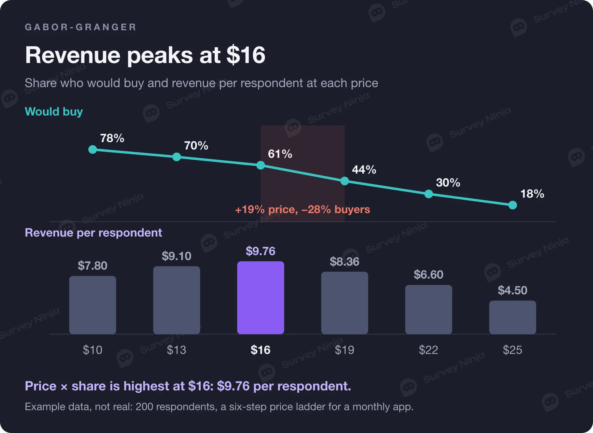
Here is a second illustrative example, not real data: 200 respondents and a six-step ladder for the same app. "Would buy" counts everyone whose highest accepted price is at or above that step.
| Price, $ | Would buy (of 200) | Share | Revenue per respondent (price × share) |
|---|---|---|---|
| 10 | 156 | 78% | $7.80 |
| 13 | 140 | 70% | $9.10 |
| 16 | 122 | 61% | $9.76 |
| 19 | 88 | 44% | $8.36 |
| 22 | 60 | 30% | $6.60 |
| 25 | 36 | 18% | $4.50 |
The share column is the demand curve. Multiply each price by its share and the highest product marks the revenue-maximizing price, here $16. Notice what happens between $16 and $19: the price rises by about 19%, while the share of buyers falls from 61% to 44%, a drop of 28%. That step is where demand turns elastic.
If you know your variable cost per customer, use margin instead of price. With a cost of $4, the margin per respondent is (16 − 4) × 61% = $7.32 at $16 and (19 − 4) × 44% = $6.60 at $19, so $16 still wins. With a cost of $8 the two are almost level, $4.88 against $4.84, and that is a sign to test both prices with real customers.
Stated purchase intent usually runs higher than real buying. Many teams count only "definitely would buy", or discount the "probably" answers, before reading the curve. Whatever rule you choose, apply it to every price step in the same way.
Van Westendorp or Gabor-Granger: which method when
Use Van Westendorp when you do not know the range yet. Use Gabor-Granger when you have a shortlist of prices and need to pick one. Many studies run Van Westendorp first and build the Gabor-Granger ladder inside the acceptable range it finds.
| Situation | Method | Why |
|---|---|---|
| New product or category, no idea of the range | Van Westendorp | Open answers show where price perception starts and ends |
| Three to seven candidate prices, need the one with the most revenue | Gabor-Granger | Gives a demand share per price and a revenue curve |
| Need both a range and a demand estimate from one survey | Van Westendorp with the Newton-Miller-Smith extension | Adds purchase likelihood at each person's own prices |
| Price depends on features and plan contents | Conjoint analysis | Trades price off against features instead of asking about price alone |
| Need to compare a few price and offer versions cleanly | Monadic test, one version per respondent | Each person sees one price, so there is no anchoring between versions |
The last row deserves a word. Showing each respondent only one price version and comparing the groups avoids the anchoring that a ladder creates. Our guide to monadic and sequential monadic tests shows how to set that up, and the same logic applies to price as to concept testing.
Who to ask and how many answers you need
Ask people who could actually buy: current customers of the category, people who match your buyer profile, decision-makers in B2B. Price perception from people outside the market is noise. If you sell to several segments, define them before fielding; our guide on how to define a target audience walks through it. Then screen out respondents who do not fit, and keep the segment as a variable so you can read the curves for each group. Define segments by how people buy and use the product, such as company size, use case or current plan, and use them to design plans and packages anyone can choose. Do not charge anyone more because of gender, ethnicity, religion, disability or another protected trait: that is discrimination, and in many places it is against the law.
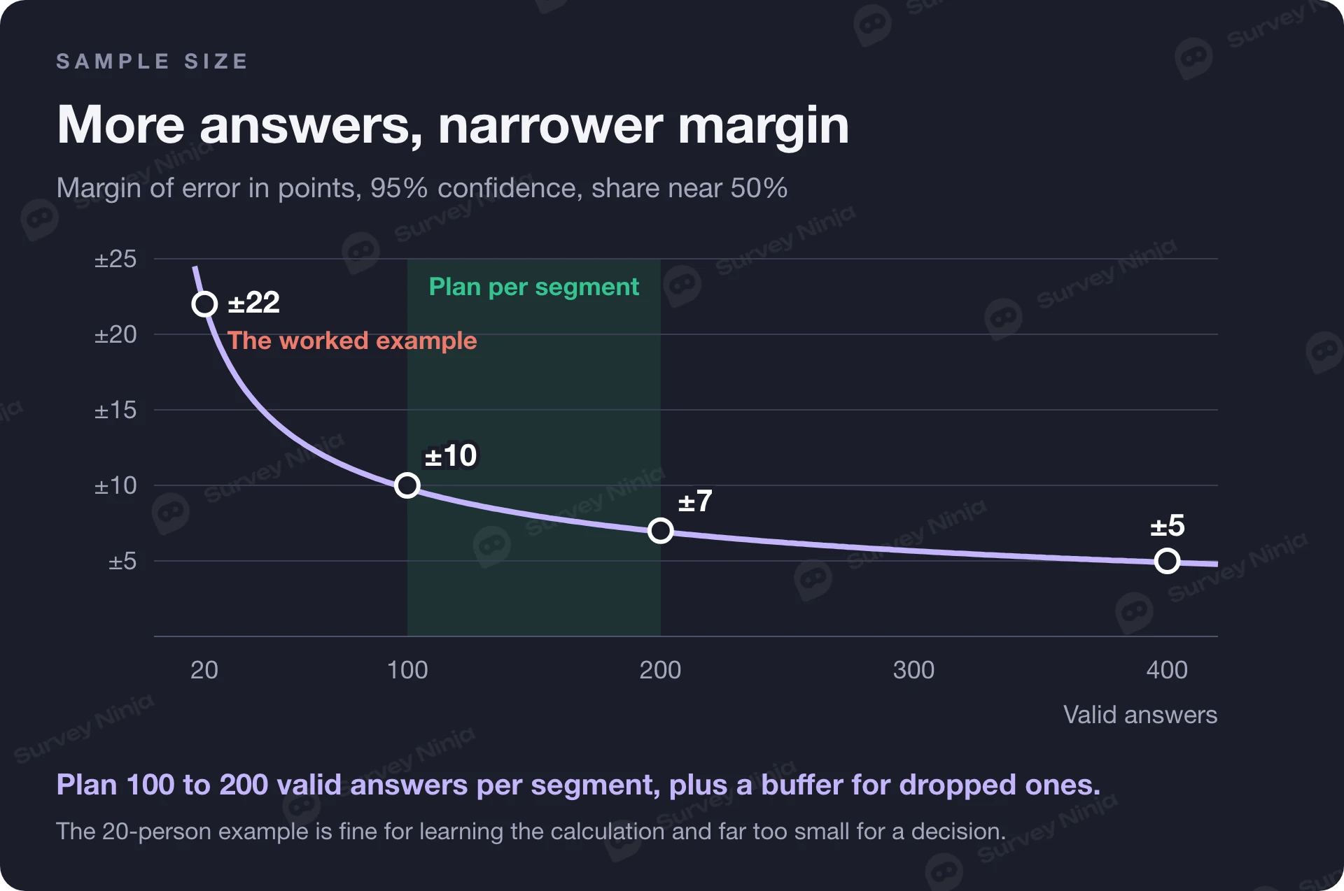
Every point on these curves is a proportion, so the usual margin of error applies. At 95% confidence and a share near 50%, 20 respondents give about ±22 points, 100 give about ±10, 200 give about ±7 and 400 give about ±5. The 20-person example above is fine for learning the calculation and far too small for a decision. Plan at least 100 to 200 valid answers per segment you want to read separately, and add a buffer for answers you will drop in the consistency check. The sample size calculator gives the number for your target precision, and the margin of error calculator tells you how precise the curves are once data is in. For an interval around any single share, use the confidence interval calculator.
Checks before you trust the numbers
Order check. Drop respondents whose four answers are not in increasing order, as in the example. Report how many you dropped. A high share, say a fifth of the sample or more, usually means the questions were confusing, the order of questions was shuffled, or the product description was unclear.
Range check. "Too expensive: $10,000" for a monthly app is a typo or a joke. Set a plausible maximum before fielding and apply it to everyone.
Rounding. People answer in round numbers, so the curves move in steps. Report crossings as a range, "$15 to $16" for the example's optimal point, rather than to the cent.
The Newton-Miller-Smith extension. Van Westendorp's method describes how people perceive price and says nothing about how many would buy. In 1993 Newton, Miller and Smith proposed an extension, presented at the American Marketing Association's Advanced Research Techniques Forum, that adds two questions: how likely the respondent is to buy at their own "bargain" price and at their own "expensive" price, usually on a five-point scale. The answers are converted to purchase probabilities. A common calibration, the default in the R package mentioned above, maps the scale to 70%, 50%, 30%, 10% and 0%, and treats the "too cheap" and "too expensive" prices as zero. Interpolating between each person's prices gives a demand curve, and price times demand gives a revenue curve from the same survey.
Limits of a pricing survey
A price survey measures what people say. Respondents pay nothing when they answer, so stated thresholds can sit far from what they do at checkout. Treat the results as a range to test, then confirm with real offers: a pricing page experiment, a limited launch or a sales conversation with a real quote. In a live test, charge every buyer the price they saw, do not show a crossed-out old price nobody ever paid, and check the consumer rules where you sell: some require you to say when a price is personalized.
Context moves the answers. Prices respondents saw recently, a competitor they have in mind, question order and the default value of an input all act as anchors. The method also sees one product in isolation, while real buyers compare alternatives, bundles and discounts. For the wider picture of who buys and why, pair the pricing study with broader market research.
How to run a pricing survey in SurveyNinja
Build the survey in the survey maker: a product description screen, then the four Van Westendorp questions as sliders, or as number questions from the Basic plan, in a fixed order. Answer piping lets you repeat a respondent's own answer in the next question, for example "You said $12 is a bargain. At what price would it start to feel expensive?", which helps people keep their answers in order. Add a screening question at the start and use screen-out logic to end the survey for people outside your market. For Gabor-Granger, skip logic moves each respondent up or down the price ladder depending on their answer.
When the answers are in, export them to XLSX, CSV or SPSS, which works on every plan, and build the curves in a spreadsheet with the formulas above. To draft questions for a specific product, start with the free price research question generator and edit the draft so it describes your product the way a buyer would see it.
Frequently asked questions
What is the Van Westendorp price sensitivity meter?
It is a pricing survey method introduced by Peter van Westendorp in 1976. Respondents name four prices: too cheap, a bargain, expensive and too expensive. Cumulative curves of the answers cross at four points, which define an acceptable price range and an optimal and an indifference price point.
What are the four Van Westendorp questions?
At what price would the product be so cheap you would doubt its quality? At what price would it be a bargain? At what price would it start to feel expensive? At what price would it be so expensive you would not consider buying it? Show a product description first and keep the order fixed.
How do you calculate the optimal price point?
Build the "too cheap" curve as the share of respondents whose too-cheap answer is at or above each price, and the "too expensive" curve as the share whose answer is at or below it. The optimal price point is where the two curves cross, found by linear interpolation between listed prices.
What is the difference between Van Westendorp and Gabor-Granger?
Van Westendorp asks open price thresholds and gives an acceptable range. Gabor-Granger shows set prices from a ladder and asks about purchase at each one, which gives a demand curve and a revenue-maximizing price. Many studies use Van Westendorp to find the range and Gabor-Granger to choose within it.
How many respondents do you need for a Van Westendorp survey?
Each curve point is a proportion, so precision depends on the sample. With 100 valid answers the margin of error is about ±10 points, with 200 about ±7. Plan 100 to 200 valid answers per segment you want to analyze, plus a buffer for respondents dropped in the consistency check.
Which respondents should you remove from a Van Westendorp analysis?
Remove anyone whose answers are not in increasing order: too cheap below bargain, bargain below expensive, expensive below too expensive. Also remove implausible values above a maximum you set before fielding. Report how many were removed, because a high share points to unclear questions.
Updated: Nov 11, 2026 Published: Nov 9, 2026